9 Multi-Dimensional Analysis

Multi-Dimensional Analysis (MDA) is a process made up of 4 main steps:

Identification of relevant variables
Extraction of factors from variables
Functional interpretation of factors as dimensions
Placement of categories on the dimensions

It is also a specific application of factor analysis. Factor analysis is a method(s) for reducing complexity in linguistic data, which can identify underlying principles of systematic variation (Biber 1988).

library(tidyverse)
library(quanteda)
library(nFactors)
library(gt)

Load functions:

library(mda.biber)

9.1 Case 1: Biber Tagger

In order to carry out MDA, we would like to have 5 times as many observations than variables. This generally precludes carrying out MDA (or factor analysis) with simple word counts. We need data that has, in some way, been tagged.

For this lab, we will use data prepared using the R package pseudobibeR, which emulates the classification system that Biber has used and reported in much of his research. The package aggregates the lexicogrammatical and functional features widely used for text-type, register, and genre classification tasks.

The scripts are not really taggers. Rather, they use udpipe or spaCy part-of-speech tagging and dependency parsing to summarize patterns. They organize 67 categories that are described here:

https://cran.r-project.org/web/packages/pseudobibeR/refman/pseudobibeR.html

For this lab, you won’t need to use the package functions. But if you’d like to try it out for any of your projects, you can follow the instructions here:

https://cran.r-project.org/web/packages/pseudobibeR/refman/pseudobibeR.html

9.1.1 The Brown Corpus

Let’s start with counts from the Brown Corpus. The Brown family of corpora is discussed on pg. 16 of Brezina. You can also find more about it here:

http://icame.uib.no/brown/bcm.html

The data is included as brown_biber and brown_meta in the cmu.textstat package:

library(cmu.textstat)

We will join the data with the metadata, in order to calculate dimension scores by register and evaluate them. Note that it must be formatted as a factor. For convenience sake, we’ll move the file names to the row names and put our factor as the first column.

brown_biber <- brown_biber |>
  left_join(dplyr::select(brown_meta, doc_id, text_type)) |>
  mutate(text_type = as.factor(text_type)) |>
  column_to_rownames("doc_id") |>
  relocate(text_type)

9.1.2 Correlation matrix

Before calculating our factors, let’s check a correlation matrix. Note that we’re dropping the first (factor) column.

bc_cor <- brown_biber |>
  select(!text_type) |>
  cor(method = "pearson")

corrplot::corrplot(bc_cor, type = "upper", order = "hclust",
         tl.col = "black", tl.srt = 45, diag = F, tl.cex = 0.5)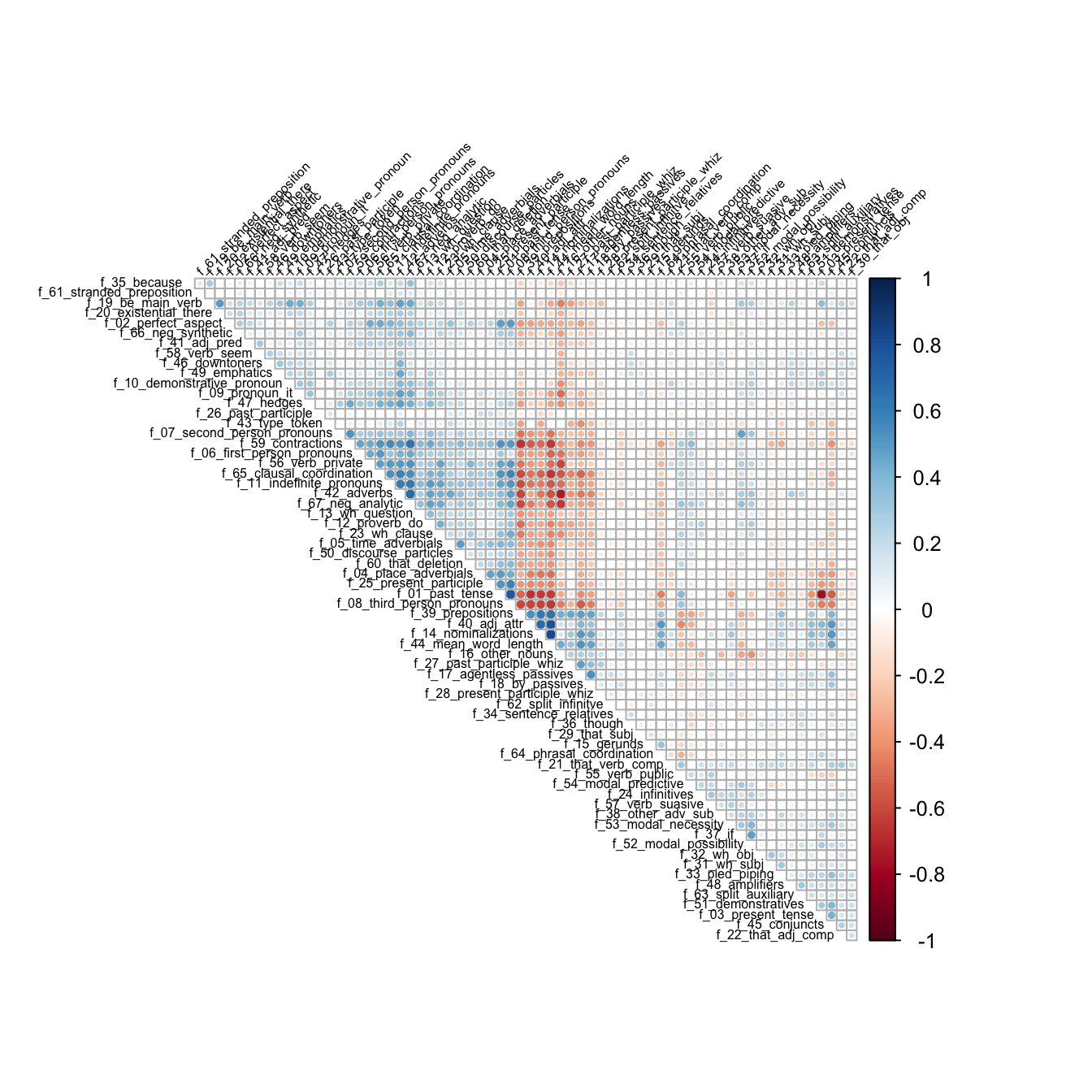

Correlation matrix of lexico-grammatical categories.

9.1.3 Determining number of factors

Typically, the number of factors is chosen after inspecting a scree plot.

screeplot_mda(brown_biber)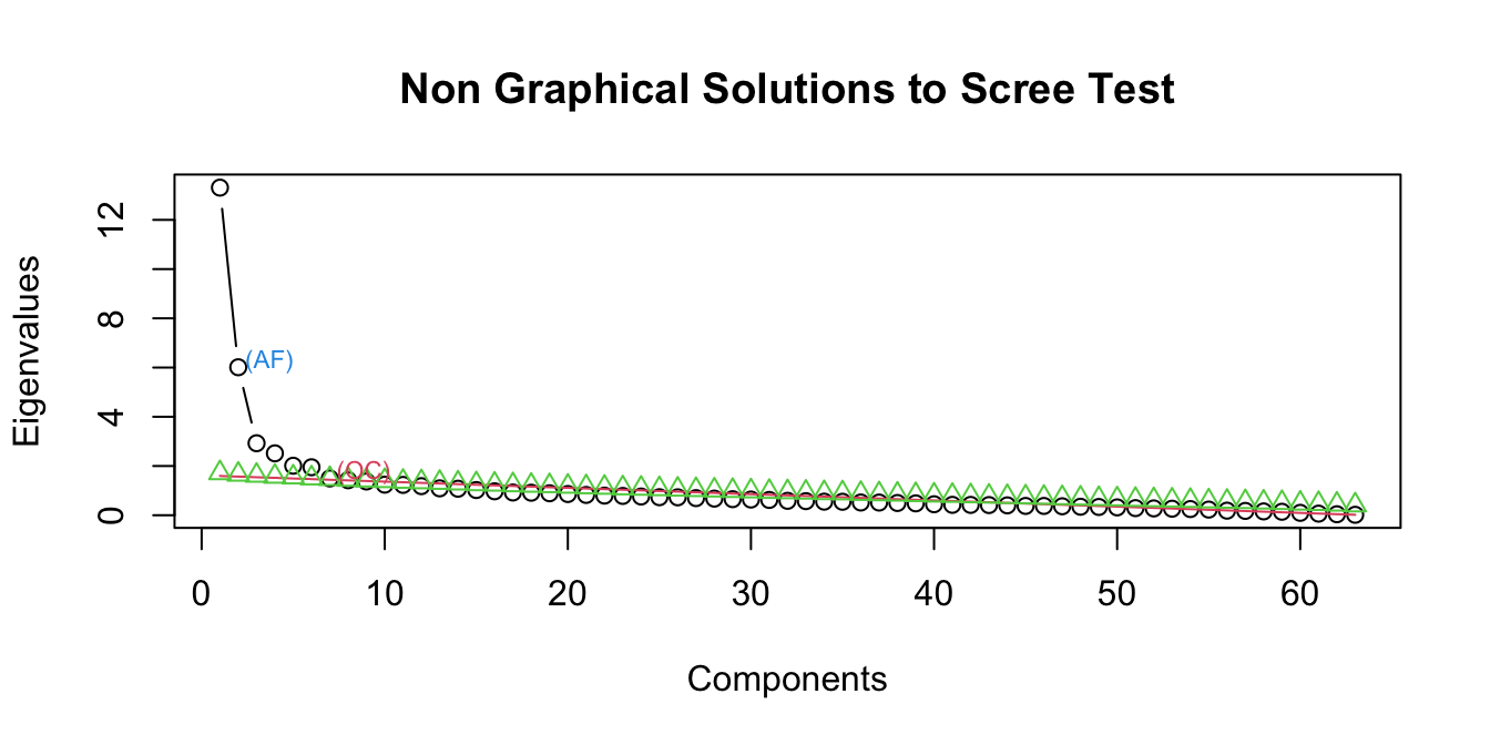

A common method for interpreting a scree plot is to look for the “bend” in the elbow, which would be 3 or 4 factors in this case. We can also look at the results of other kinds of solutions like optimal coordinates, which measures the gradients associated with eigenvalues and their preceding coordinates, and acceleration factor, which determines the coordinate where the slope of the curve changes most abruptly. In this case OC suggests 6 factors and AF 1.

For the purposes of this exercise, we’ll start with 3 factors.

9.1.4 Calculating factor loadings and MDA scores

In factor analysis factors so that they pass through the middle of the relevant variables. For linguistic variable it is conventional to use a promax rotation (see Brezina pgs. 164-167). There is also a nice explanation of rotations here:

https://personal.utdallas.edu/~herve/Abdi-rotations-pretty.pdf

To place our categories along the dimensions, data is standardized by converting to z-scores. For each text, a dimension score is calculated by summing all of the high-positive variables subtracting all of the high-negative variables. Then, the mean is calculated for each category.

For these calculations, we will use the mda_loadings() function.

bc_mda <- mda_loadings(brown_biber, n_factors = 3)

We can access factor loadings and group means through attributes.

attr(bc_mda, 'loadings') |>
  rownames_to_column("Feature") |>
  gt() |>
  fmt_number(
    columns = everything(),
    decimals = 2
  )

Factor loadings for the Brown Corpus.
Feature	Factor1	Factor2	Factor3
f_01_past_tense	−0.15	1.10	0.16
f_02_perfect_aspect	0.05	0.52	0.28
f_03_present_tense	0.60	−1.06	−0.04
f_04_place_adverbials	0.17	0.42	−0.11
f_05_time_adverbials	0.23	0.32	0.06
f_06_first_person_pronouns	0.44	0.15	0.22
f_07_second_person_pronouns	0.66	−0.11	−0.14
f_08_third_person_pronouns	0.19	0.73	0.16
f_09_pronoun_it	0.32	0.11	0.39
f_10_demonstrative_pronoun	0.36	−0.15	0.37
f_11_indefinite_pronouns	0.49	0.30	0.26
f_12_proverb_do	0.54	0.04	0.14
f_13_wh_question	0.39	0.10	0.05
f_14_nominalizations	−0.51	−0.39	0.21
f_15_gerunds	−0.02	−0.16	−0.03
f_16_other_nouns	−0.29	−0.32	−0.77
f_17_agentless_passives	−0.48	−0.21	0.00
f_18_by_passives	−0.45	−0.16	0.02
f_19_be_main_verb	0.46	−0.09	0.41
f_20_existential_there	0.13	0.13	0.30
f_21_that_verb_comp	−0.18	0.08	0.44
f_22_that_adj_comp	0.01	−0.10	0.38
f_23_wh_clause	0.36	0.23	0.22
f_24_infinitives	0.10	0.01	0.24
f_25_present_participle	0.12	0.48	−0.03
f_27_past_participle_whiz	−0.53	0.08	−0.11
f_28_present_participle_whiz	−0.22	0.03	−0.16
f_30_that_obj	0.00	−0.11	0.26
f_31_wh_subj	−0.14	−0.10	0.14
f_32_wh_obj	−0.03	0.04	0.27
f_33_pied_piping	−0.17	−0.17	0.34
f_34_sentence_relatives	−0.21	−0.07	0.08
f_35_because	0.33	−0.13	0.15
f_36_though	−0.20	0.16	0.32
f_37_if	0.53	−0.27	0.12
f_38_other_adv_sub	0.02	−0.06	0.33
f_39_prepositions	−0.68	−0.23	−0.06
f_40_adj_attr	−0.41	−0.47	0.18
f_41_adj_pred	0.14	0.16	0.26
f_42_adverbs	0.57	0.21	0.51
f_43_type_token	0.14	0.12	−0.06
f_44_mean_word_length	−0.65	−0.36	0.04
f_45_conjuncts	−0.20	−0.41	0.37
f_46_downtoners	0.13	−0.03	0.38
f_47_hedges	0.40	0.10	0.24
f_48_amplifiers	0.04	−0.11	0.36
f_49_emphatics	0.41	−0.26	0.26
f_50_discourse_particles	0.41	0.07	0.00
f_51_demonstratives	−0.10	−0.31	0.31
f_52_modal_possibility	0.45	−0.39	0.29
f_53_modal_necessity	0.10	−0.36	0.19
f_54_modal_predictive	0.43	−0.12	−0.09
f_55_verb_public	0.07	0.38	0.09
f_56_verb_private	0.25	0.44	0.44
f_57_verb_suasive	−0.12	0.03	0.03
f_58_verb_seem	−0.02	0.13	0.39
f_59_contractions	0.61	0.25	−0.03
f_60_that_deletion	0.25	0.26	0.03
f_63_split_auxiliary	−0.04	−0.07	0.37
f_64_phrasal_coordination	−0.15	−0.39	−0.02
f_65_clausal_coordination	0.47	0.37	0.28
f_66_neg_synthetic	0.07	0.32	0.35
f_67_neg_analytic	0.57	0.20	0.38

9.1.5 Plotting the results

The means are conventionally positioned on a stick plot of the kind Brezina shows on pg. 169.

stickplot_mda(bc_mda, n_factor = 1)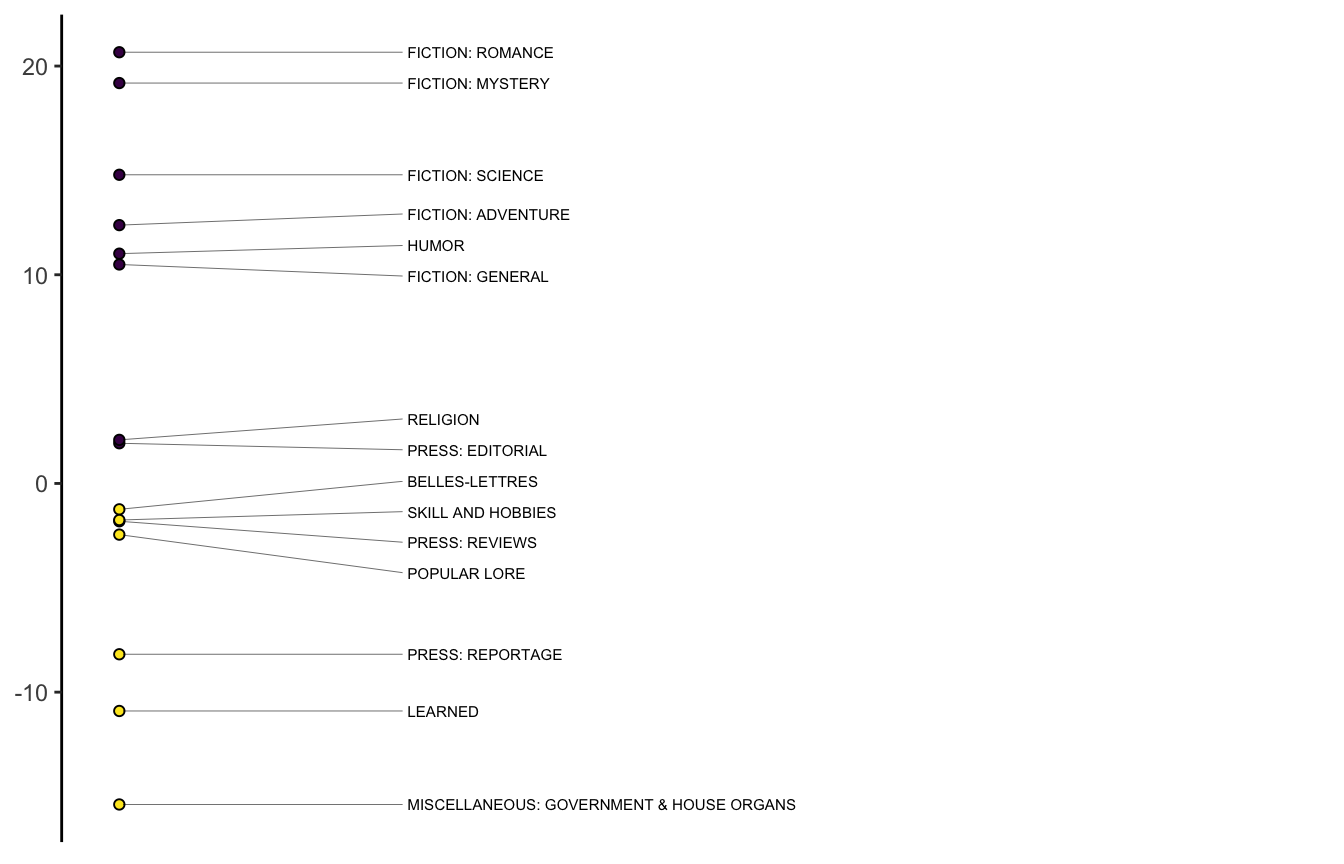

Dimension score means by discipline plotted along Factor 1.

We can also show the same plot with the factor loadings.

heatmap_mda(bc_mda, n_factor = 1)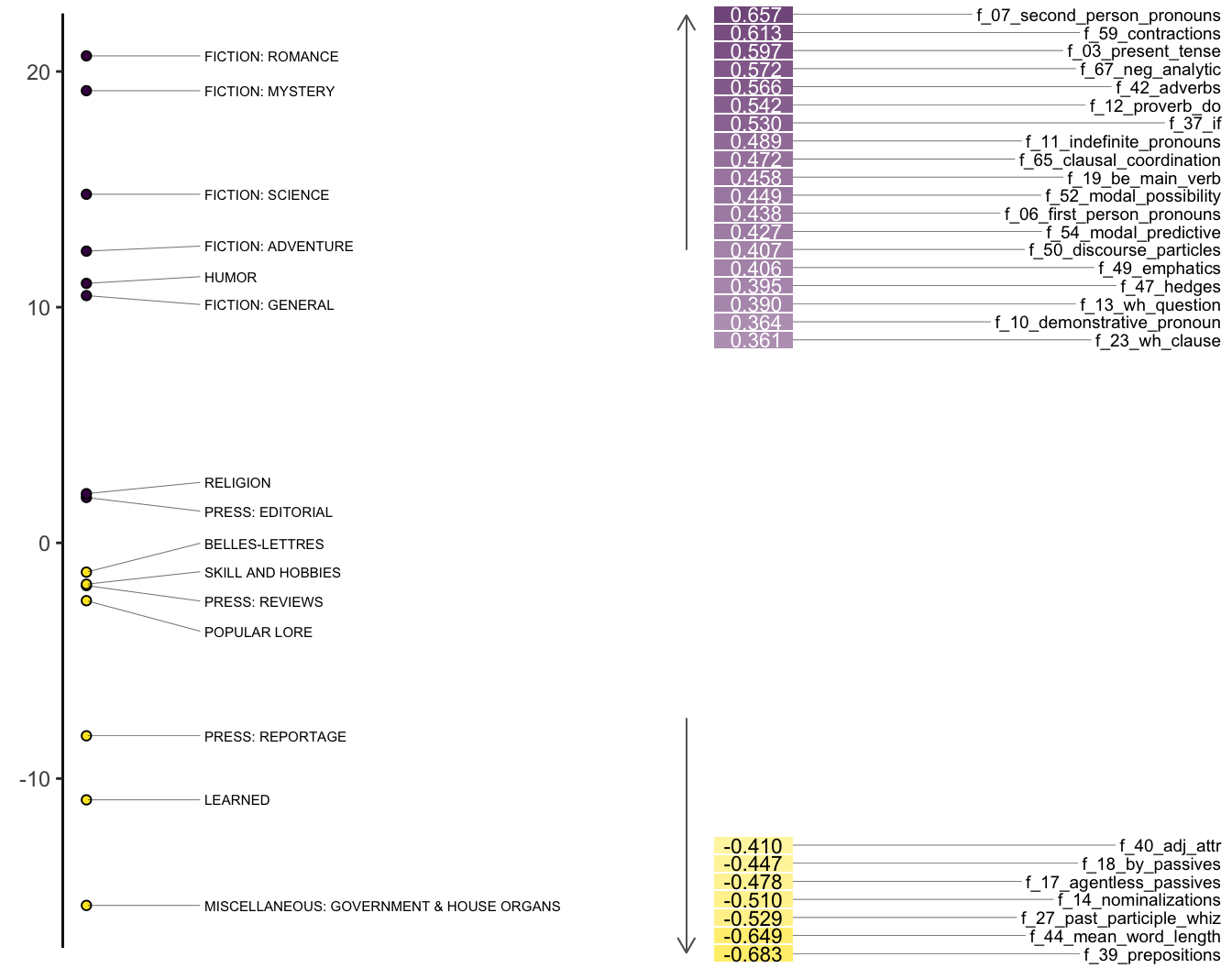

9.1.6 Evaluating MDA

Typically, MDA is evaluated using ANOVA, reporting the F statistic, degrees of freedom, and R-squared. We can extract that information from a linear model.

f_aov <- aov(Factor1 ~ group, data = bc_mda)
broom::tidy(f_aov)

# A tibble: 2 × 6
  term         df  sumsq meansq statistic   p.value
  <chr>     <dbl>  <dbl>  <dbl>     <dbl>     <dbl>
1 group        14 51553.  3682.      32.1  3.49e-60
2 Residuals   485 55651.   115.      NA   NA

gtsummary::tbl_regression(lm(Factor1 ~ group, data = bc_mda)) |>
  gtsummary::add_glance_source_note() |>
  gtsummary::as_gt()

Characteristic	Beta	95% CI	p-value
group
BELLES-LETTRES	—	—
FICTION: ADVENTURE	14	9.0, 18	<0.001
FICTION: GENERAL	12	7.1, 16	<0.001
FICTION: MYSTERY	20	15, 25	<0.001
FICTION: ROMANCE	22	17, 27	<0.001
FICTION: SCIENCE	16	7.1, 25	<0.001
HUMOR	12	4.8, 20	0.001
LEARNED	-9.7	-13, -6.3	<0.001
MISCELLANEOUS: GOVERNMENT & HOUSE ORGANS	-14	-19, -9.6	<0.001
POPULAR LORE	-1.2	-5.1, 2.7	0.5
PRESS: EDITORIAL	3.2	-1.6, 7.9	0.2
PRESS: REPORTAGE	-6.9	-11, -2.9	<0.001
PRESS: REVIEWS	-0.57	-6.2, 5.1	0.8
RELIGION	3.3	-2.3, 9.0	0.2
SKILL AND HOBBIES	-0.51	-4.8, 3.8	0.8
Abbreviation: CI = Confidence Interval
R² = 0.481; Adjusted R² = 0.466; Sigma = 10.7; Statistic = 32.1; p-value = <0.001; df = 14; Log-likelihood = -1,888; AIC = 3,807; BIC = 3,874; Deviance = 55,651; Residual df = 485; No. Obs. = 500

gtsummary::tbl_regression(lm(Factor2 ~ group, data = bc_mda)) |>
  gtsummary::add_glance_source_note() |>
  gtsummary::as_gt()

Characteristic	Beta	95% CI	p-value
group
BELLES-LETTRES	—	—
FICTION: ADVENTURE	15	12, 17	<0.001
FICTION: GENERAL	13	11, 16	<0.001
FICTION: MYSTERY	14	12, 17	<0.001
FICTION: ROMANCE	14	12, 17	<0.001
FICTION: SCIENCE	8.1	3.3, 13	0.001
HUMOR	7.3	3.2, 11	<0.001
LEARNED	-7.8	-9.6, -5.9	<0.001
MISCELLANEOUS: GOVERNMENT & HOUSE ORGANS	-9.6	-12, -7.1	<0.001
POPULAR LORE	-0.58	-2.7, 1.5	0.6
PRESS: EDITORIAL	-2.3	-4.8, 0.28	0.081
PRESS: REPORTAGE	0.71	-1.5, 2.9	0.5
PRESS: REVIEWS	-2.9	-6.0, 0.18	0.065
RELIGION	-3.8	-6.9, -0.75	0.015
SKILL AND HOBBIES	-5.6	-7.9, -3.2	<0.001
Abbreviation: CI = Confidence Interval
R² = 0.662; Adjusted R² = 0.652; Sigma = 5.82; Statistic = 67.7; p-value = <0.001; df = 14; Log-likelihood = -1,582; AIC = 3,196; BIC = 3,264; Deviance = 16,404; Residual df = 485; No. Obs. = 500

gtsummary::tbl_regression(lm(Factor3 ~ group, data = bc_mda)) |>
  gtsummary::add_glance_source_note() |>
  gtsummary::as_gt()

Characteristic	Beta	95% CI	p-value
group
BELLES-LETTRES	—	—
FICTION: ADVENTURE	-0.81	-3.7, 2.1	0.6
FICTION: GENERAL	-0.23	-3.1, 2.7	0.9
FICTION: MYSTERY	3.1	-0.02, 6.2	0.051
FICTION: ROMANCE	2.9	0.02, 5.8	0.048
FICTION: SCIENCE	5.4	-0.21, 11	0.059
HUMOR	2.9	-1.7, 7.6	0.2
LEARNED	-0.11	-2.2, 2.0	>0.9
MISCELLANEOUS: GOVERNMENT & HOUSE ORGANS	-9.2	-12, -6.3	<0.001
POPULAR LORE	-2.4	-4.8, 0.09	0.059
PRESS: EDITORIAL	-0.87	-3.8, 2.1	0.6
PRESS: REPORTAGE	-10	-13, -7.8	<0.001
PRESS: REVIEWS	-3.9	-7.4, -0.29	0.034
RELIGION	4.3	0.73, 7.9	0.018
SKILL AND HOBBIES	-5.1	-7.8, -2.4	<0.001
Abbreviation: CI = Confidence Interval
R² = 0.273; Adjusted R² = 0.252; Sigma = 6.76; Statistic = 13.0; p-value = <0.001; df = 14; Log-likelihood = -1,657; AIC = 3,346; BIC = 3,414; Deviance = 22,146; Residual df = 485; No. Obs. = 500

9.2 Case 2: DocuScope

Unlike the Biber tagger, DocuScope is a dictionary-based tagger. It has been developed at CMU by David Kaufer and Suguru Ishizaki since the early 2000s. You can find the dictionary categories described here:

https://docuscospacy.readthedocs.io/en/latest/docuscope.html#categories

9.2.1 Load the dictionary

A simplified version of the DocuScope dictionary is included in quanteda.extras. We’ll also use micusp_mini from cmu.textstat.

library(quanteda.extras)
library(cmu.textstat)

DocuScope is a very large dictionary (or lexicon) that organizes tens of millions of words and phrases into rhetorically oriented categories. It has some overlap with a few Biber’s functional categories (like hedges), but is fundamentally different, as it isn’t bases on parts-of-speech.

The ds_dict is a small quanteda dictionary that organizes a smaller set of words of phrases (tens of thousands rather than tens of millions). Here is a sample from 3 of the categories:

ds_dict[1:3]

Dictionary object with 3 key entries.
- [AcademicTerms]:
  - a chapter in, a couple, a declaration of, a detail, a distinction between, a domain, a force, a forced, a form of, a grade, a hint of, a home for, a hub, a kind of, a kind of a, a load, a loaded, a metaphor for, a mix of, a mixture of [ ... and 8,884 more ]
- [AcademicWritingMoves]:
  - . in this article ,, . in this paper, . this essay, . this paper, . this report, . this work, . to avoid, a better understanding, a common problem, a debate about, a debate over, a first step, a goal of, a great deal of attention, a huge problem, a key to, a major problem, a method of, a notion that, a number of studies [ ... and 1,141 more ]
- [Character]:
  - ; block, ; bring, ; call, ; center, ; check, ; chill, ; close, ; color, ; control, ; cook, ; cool, ; cover, ; cross, ; cut, ; design, ; discard, ; don, ; down, ; drain, ; e-mail [ ... and 18,754 more ]

9.2.2 Tokenize the corpus

Again, we will use the **micusp_mini*, and we’ll begin by tokenizing the data. Note that we’re retaining as much of the original data as possible including punctuation. This is because our dictionary includes punctuation marks in it’s entries.

micusp_tokens <- micusp_mini |>
  corpus() |>
  tokens(remove_punct = FALSE, remove_numbers = FALSE, 
         remove_symbols = FALSE, what = "word")

Next, we will use the tokens_lookup() function to count and categorize our features.

ds_counts <- micusp_tokens |>
  tokens_lookup(dictionary = ds_dict, levels = 1, valuetype = "fixed") |>
  dfm() |>
  convert(to = "data.frame") |>
  as_tibble()

Finally, we need to normalize the counts. Because DocuScope is not categorizing ALL of our tokens, we need a total count from the original tokens object.

tot_counts <- data.frame(tot_counts = quanteda::ntoken(micusp_tokens)) |>
  tibble::rownames_to_column("doc_id") |>
  dplyr::as_tibble()

ds_counts <- dplyr::full_join(ds_counts, tot_counts, by = "doc_id")

Now we can normalize by the total counts before preparing the data for factor analysis.

ds_counts <- ds_counts |>
  dplyr::mutate_if(is.numeric, list(~./tot_counts), na.rm = TRUE) |>
  dplyr::mutate_if(is.numeric, list(~.*100), na.rm = TRUE) |>
  dplyr::select(-tot_counts)

ds_counts <- ds_counts |>
  mutate(text_type = str_extract(doc_id, "^[A-Z]+")) |>
  mutate(text_type = as.factor(text_type)) |>
  column_to_rownames("doc_id")

9.2.3 Calculating factor loadings and MDA score

Again, we will use 3 factors.

micusp_mda <- mda_loadings(ds_counts, n_factors = 3)

9.2.4 Evaluating MDA

We can again check to see how explanatory our dimensions are.

gtsummary::tbl_regression(lm(Factor1 ~ group, data = micusp_mda)) |>
  gtsummary::add_glance_source_note() |>
  gtsummary::as_gt()

Characteristic	Beta	95% CI	p-value
group
BIO	—	—
CEE	-4.3	-7.3, -1.3	0.005
CLS	7.7	4.8, 11	<0.001
ECO	0.40	-2.6, 3.4	0.8
EDU	5.8	2.9, 8.8	<0.001
ENG	10	7.3, 13	<0.001
HIS	4.8	1.8, 7.8	0.002
IOE	-0.29	-3.3, 2.7	0.8
LIN	2.8	-0.19, 5.7	0.066
MEC	-4.8	-7.8, -1.9	0.002
NRE	0.20	-2.8, 3.2	0.9
NUR	3.4	0.40, 6.3	0.026
PHI	9.5	6.5, 12	<0.001
PHY	-1.9	-4.9, 1.1	0.2
POL	6.0	3.0, 9.0	<0.001
PSY	3.2	0.20, 6.1	0.037
SOC	5.1	2.2, 8.1	<0.001
Abbreviation: CI = Confidence Interval
R² = 0.646; Adjusted R² = 0.609; Sigma = 3.36; Statistic = 17.5; p-value = <0.001; df = 16; Log-likelihood = -438; AIC = 912; BIC = 969; Deviance = 1,722; Residual df = 153; No. Obs. = 170

gtsummary::tbl_regression(lm(Factor2 ~ group, data = micusp_mda)) |>
  gtsummary::add_glance_source_note() |>
  gtsummary::as_gt()

Characteristic	Beta	95% CI	p-value
group
BIO	—	—
CEE	-1.2	-4.7, 2.3	0.5
CLS	-7.6	-11, -4.1	<0.001
ECO	-3.3	-6.8, 0.24	0.067
EDU	-2.9	-6.4, 0.65	0.11
ENG	-8.2	-12, -4.7	<0.001
HIS	-10	-14, -6.5	<0.001
IOE	-4.0	-7.5, -0.53	0.024
LIN	-0.51	-4.0, 3.0	0.8
MEC	-1.3	-4.8, 2.2	0.5
NRE	-8.4	-12, -4.9	<0.001
NUR	-3.3	-6.8, 0.16	0.061
PHI	-1.6	-5.1, 1.9	0.4
PHY	-1.0	-4.5, 2.5	0.6
POL	-13	-17, -9.7	<0.001
PSY	-1.3	-4.8, 2.2	0.5
SOC	-7.2	-11, -3.7	<0.001
Abbreviation: CI = Confidence Interval
R² = 0.506; Adjusted R² = 0.454; Sigma = 3.96; Statistic = 9.78; p-value = <0.001; df = 16; Log-likelihood = -466; AIC = 969; BIC = 1,025; Deviance = 2,405; Residual df = 153; No. Obs. = 170

gtsummary::tbl_regression(lm(Factor3 ~ group, data = micusp_mda)) |>
  gtsummary::add_glance_source_note() |>
  gtsummary::as_gt()

Characteristic	Beta	95% CI	p-value
group
BIO	—	—
CEE	0.18	-2.5, 2.9	0.9
CLS	-1.7	-4.4, 0.96	0.2
ECO	3.5	0.84, 6.2	0.010
EDU	3.0	0.29, 5.6	0.030
ENG	-2.2	-4.9, 0.49	0.11
HIS	-3.2	-5.9, -0.55	0.019
IOE	3.4	0.75, 6.1	0.012
LIN	-0.97	-3.6, 1.7	0.5
MEC	-0.50	-3.2, 2.2	0.7
NRE	3.0	0.37, 5.7	0.026
NUR	5.2	2.6, 7.9	<0.001
PHI	-0.73	-3.4, 1.9	0.6
PHY	-1.3	-4.0, 1.4	0.3
POL	1.5	-1.2, 4.2	0.3
PSY	0.08	-2.6, 2.8	>0.9
SOC	-0.04	-2.7, 2.6	>0.9
Abbreviation: CI = Confidence Interval
R² = 0.387; Adjusted R² = 0.322; Sigma = 3.02; Statistic = 6.03; p-value = <0.001; df = 16; Log-likelihood = -420; AIC = 877; BIC = 933; Deviance = 1,398; Residual df = 153; No. Obs. = 170

9.2.5 Plotting the results

And we can plot the first factor.

heatmap_mda(micusp_mda, n_factor = 1)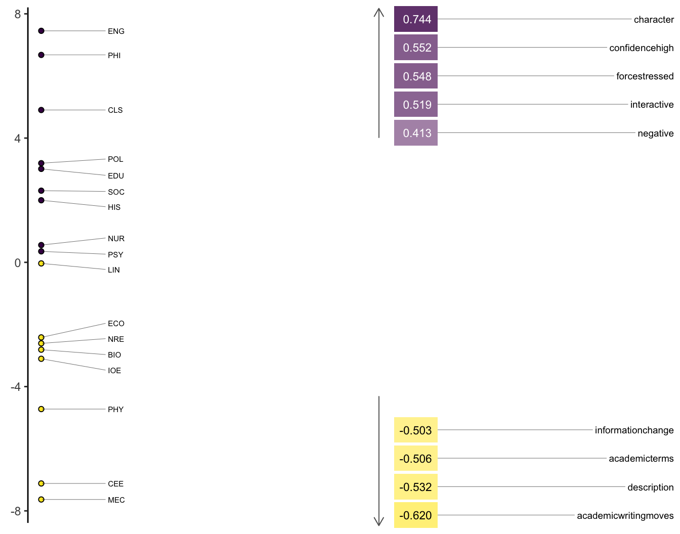

9.2.6 Interpreting the factors as dimensions

The functional interpretation of factors as dimensions (Brezina pgs. 167-168) is probably the most challenging part of MDA. As analysts, we need to make sense out of why features (whether parts-of-speech, rhetorical categories, or other measures) are grouping together and contributing to the patterns of variation evident in products of the analysis.

That interpretation usually involves giving names to the dimensions based on their constituent structures. In Biber’s original study, he called his first, most explanatory dimension Involved vs. Informational Production. At the positive (Involved) end of the dimension are telephone and face-to-face conversations. At the negative (Information) end are official documents and academic prose.

Features with high positive loadings include private verbs (like think), contractions, and first and second person pronouns. Features with high negative loadings include nouns and propositional phrases. Biber concludes that these patterns reflect the communicative purposes of the registers. Ones that are more interactive and affective vs. others that are more instructive and informative.

In order to understand how certain features are functioning, it is important to see how they are being used, which we can do effienciently with Key Words in Context (KWIC). Here we take “Confidence High” from the positive end of the dimension and “Academic Writing Moves” from the negative.

ch <- kwic(micusp_tokens, ds_dict["ConfidenceHigh"])

awm <- kwic(micusp_tokens, ds_dict["AcademicWritingMoves"])

Code

ch |>
  head(10) |>
  gt()

docname	from	to	pre	keyword	post	pattern
BIO.G0.02.1	193	193	sympatry ; do these examples	simply	represent another head on the	ConfidenceHigh
BIO.G0.02.1	405	406	speciation in this genus ,	most likely	under sympatric conditions . The	ConfidenceHigh
BIO.G0.02.1	712	712	that this mechanism is not	very	efficient , and depends on	ConfidenceHigh
BIO.G0.02.1	1151	1151	normal host species respond in	predictable	manners : choosing to mate	ConfidenceHigh
BIO.G0.02.1	1436	1437	explored later ; however ,	it is	important to note here that	ConfidenceHigh
BIO.G0.02.1	1731	1731	of finding a mate that	knows	the same song as you	ConfidenceHigh
BIO.G0.02.1	1731	1732	of finding a mate that	knows the	same song as you may	ConfidenceHigh
BIO.G0.02.1	1755	1755	assume that many colonization events	probably	occurred - - only to	ConfidenceHigh
BIO.G0.02.1	1782	1782	. , 2004 ) .	Conclusively	showing that the observed diversification	ConfidenceHigh
BIO.G0.02.1	1897	1897	upon genetic data - -	obvious	arguments against this methodology and	ConfidenceHigh

Code

awm |>
  head(10) |>
  gt()

docname	from	to	pre	keyword	post	pattern
BIO.G0.02.1	260	262	, yet another possible example	has been described	by science , which may	AcademicWritingMoves
BIO.G0.02.1	598	600	, this type of behavior	has been observed	in the indigobirds of Vidua	AcademicWritingMoves
BIO.G0.02.1	920	921	( Lonchura striata ) .	They conducted	a second experiment in 2000	AcademicWritingMoves
BIO.G0.02.1	946	947	1998 study . Their experiment	was designed	principally to test three hypotheses	AcademicWritingMoves
BIO.G0.02.1	1027	1028	, the Bengalese , finch	were used	. In the cross-foster experiments	AcademicWritingMoves
BIO.G0.02.1	1213	1214	before fledging - - this	finding is	also consistent with Payne et	AcademicWritingMoves
BIO.G0.02.1	1235	1237	brood parasitizing bird species ,	these results are	unique to the Vidua .	AcademicWritingMoves
BIO.G0.02.1	1236	1237	parasitizing bird species , these	results are	unique to the Vidua .	AcademicWritingMoves
BIO.G0.02.1	1416	1417	- - implying that this	experimental data	is supported by observational studies	AcademicWritingMoves
BIO.G0.02.1	1417	1418	- implying that this experimental	data is	supported by observational studies .	AcademicWritingMoves

9.3 Works cited

Biber, Douglas. 1988. Variation Across Speech and Writing. Cambridge University Press. https://doi.org/10.1017/CBO9780511621024.