4  Distributions

4.1 Prepare a corpus

4.1.1 Load the needed packages

library(gt)
library(quanteda)
library(quanteda.textstats)
library(tidyverse)

4.1.2 Load a corpus

The repository comes with some data sets. The conventional way to format text data prior to processing is as a table with a column of document ids (which correspond to the the file names) and a column of texts. Such a table is easy to create from text data on your own local drive using the package readtext.

load("../data/sample_corpus.rda")
load("../data/multiword_expressions.rda")

To peek at the data, we’ll look at the first 100 characters in the “text” column of the first row:

sample_corpus |>
  mutate(text = substr(text, start = 1, stop = 100)) |>
  head(10) |>
  gt()

doc_id	text
acad_01	Teachers and other school personnel are often counseled to use research findings in making curricula
acad_02	Abstract Does the conflict in El Salvador, conceptualized by the U.S. government as a battle in the
acad_03	January 17, 1993, will mark the 100th anniversary of the deposing of the Hawaiian monarchy. "Prior t
acad_04	Thirty years have passed since the T1961 meeting of the National Council for the Social Studies in C
acad_05	ABSTRACT -- A common property resource with open access, such as a fishery, will be used to excess w
acad_06	Despite some encouraging signs and hopeful expectations that democracy has made reasonable progress
acad_07	evaluation component. Similarly, Stewart ( 1982,1989 ) has shown that a common response to unfamilia
acad_08	Section: Education "A lab is where you do science" ( Thornton 1972 ). An investigative laboratory (
acad_09	In 1968, the thirtieth anniversary issue of the Journal of Politics celebrated the great advance in
acad_10	monologue -- and of Novas Calvo's story -- may thus be clarified, not as that of facilitating an obj

4.1.3 Load functions

The repository also contains a number of useful functions. Here, will load some that will calculate a number of common dispersion measures.

source("../R/dispersion_functions.R")
source("../R/helper_functions.R")

4.1.4 Create and corpus

Make a corpus object.

sc <- corpus(sample_corpus)

And check the result:

sc |>
  summary() |>
  head(10) |>
  gt()

Table 4.1: Partial summary of sample corpus.

Text	Types	Tokens	Sentences
acad_01	842	2818	95
acad_02	983	2845	88
acad_03	968	2885	126
acad_04	1017	2864	102
acad_05	914	2837	109
acad_06	1007	2813	86
acad_07	663	2952	92
acad_08	870	2830	118
acad_09	980	2899	131
acad_10	1118	2883	77

4.2 Document variables (Name your files systematically!)

Important

File names can encode important meta-data. In this case, the names include text-types, much like the Corpus of Contemporary American English.

This is extremely important. When you build your own corpora, you want to purposefully and systematically name your files and organize your directories. This will save you time and effort later in your analysis.

We are now going to extract the meta-data from the file names and pass them as a variable.

doc_categories <- str_extract(sample_corpus$doc_id, "^[a-z]+")

Check the result:

Document categories.

doc_cats
acad
blog
fic
mag
news
spok
tvm
web

We will now assign the variable to the corpus. The following command might look backwards, with the function on the left hand side of the <- operator. That is because it’s an accessor function, which lets us add or modify data in an object. You can tell when a function is an accessor function like this because its help file will show that you can use it with <-, for example in ?docvars.

docvars(sc, field = "text_type") <- doc_categories

And check the summary again:

sc |>
  summary() |>
  head(10) |>
  gt()

Partial summary of sample corpus.

Text	Types	Tokens	Sentences	text_type
acad_01	842	2818	95	acad
acad_02	983	2845	88	acad
acad_03	968	2885	126	acad
acad_04	1017	2864	102	acad
acad_05	914	2837	109	acad
acad_06	1007	2813	86	acad
acad_07	663	2952	92	acad
acad_08	870	2830	118	acad
acad_09	980	2899	131	acad
acad_10	1118	2883	77	acad

Warning

Assigning docvars is based entirely on ordering. In other words, you are simply attaching a vector of categories to the corpus object. There is no merging by shared keys. Thus, you always need to be sure that your docvars are in the same order as your doc_ids. This is the reason why we extracted them directly from the doc_ids.

4.3 Tokenize the corpus

We’ll use quanteda to tokenize. And after tokenization, we’ll convert them to lower case. Why do that here? As a next step, we’ll being combining tokens like a and lot into single units. And we’ll be using a list of expressions that isn’t case sensitive.

sc_tokens <- tokens(sc, include_docvars=TRUE, remove_punct = TRUE, remove_numbers = TRUE, remove_symbols = TRUE, what = "word")

sc_tokens <- tokens_tolower(sc_tokens)

4.4 Multi-word Expressions

An issue that we run into frequently with corpus analysis is what to do with multi-word expressions. For example, consider a common English quantifier: “a lot”. Typical tokenization rules will split this into two tokens: a and lot. But counting a lot as a single unit might be important depending on our task. We have a way of telling quanteda to account for these tokens.

All that we need is a list of multi-word expressions.

The cmu.textstat comes with an example of an mwe list called multiword_expressions:

Examples of multi-word expressions.

winter haven

with a view to

with reference to

with regard to

with relation to

with respect to

The tokens_compound() function looks for token sequences that match our list and combines them using an underscore.

sc_tokens <- tokens_compound(sc_tokens, pattern = phrase(multiword_expressions))

4.5 Create a document-feature matrix

With our tokens object we can now create a document-feature-matrix using the dfm() function. As a reminder, a dfm is table with one row per document in the corpus, and one column per unique token in the corpus. Each cell contains a count of how many times a token shows up in that document.

sc_dfm <- dfm(sc_tokens)

Next we’ll create a dfm with proportionally weighted counts.

prop_dfm <- dfm_weight(sc_dfm, scheme = "prop")

4.6 Token distributions

4.6.1 Distributions of the

Let’s start by selecting frequencies of the most common token in the corpus:

freq_df <- textstat_frequency(sc_dfm) %>%
  data.frame(stringsAsFactors = F)

freq_df |>
  head(10) |>
  gt()

The 10 most frequent tokens in the sample corpus.

feature	frequency	rank	docfreq	group
the	50920	1	399	all
and	25232	2	398	all
to	24753	3	397	all
of	22060	4	399	all
a	21614	5	398	all
in	15969	6	399	all
i	12568	7	348	all
that	12537	8	396	all
you	10951	9	341	all
is	9901	10	389	all

From the weighted dfm, we can select any token that we’d like to look at more closely. In this case, we’ll select the most frequent token: the.

After selecting the variable, we will convert the data into a more friendly data structure.

There are easier ways of doing this, but the first bit of the code-chunk allows us to filter by rank and return a character vector that we can pass. This way, we can find a word of any arbitrary rank.

Also note how the rename() function is set up. Let’s say our token is the. The dfm_select() function would result with a column named the that we’d want to rename RF. So our typical syntax would be: rename(RF = the). In the chunk below, however, our column name is the variable word. To pass that variable to rename, we use !!name(word).

word <- freq_df %>% 
  filter(rank == 1) %>% 
  dplyr::select(feature) %>%
  as.character()

word_df <- dfm_select(prop_dfm, word, valuetype = "fixed") # select the token

word_df <- word_df %>% 
  convert(to = "data.frame") %>% 
  cbind(docvars(word_df)) %>% 
  rename(RF = !!as.name(word)) %>% 
  mutate(RF = RF*1000000)

With that data it is a simple matter to generate basic summary statistics using the group_by() function:

summary_table <- word_df %>% 
  group_by(text_type) %>%
  summarize(MEAN = mean(RF),
              SD = sd(RF),
              N = n())

summary_table |>
  gt()

Means and standard deviations by text-type.

text_type	MEAN	SD	N
acad	68619.64	18327.10	50
blog	51270.54	13389.38	50
fic	54202.41	14254.79	50
mag	57117.76	13986.30	50
news	50574.84	18333.09	50
spok	42693.44	9727.79	50
tvm	32532.85	11981.88	50
web	60592.68	21641.35	50

And we can inspect a histogram of the frequencies. To set the width of our bins we’ll use the Freedman-Diaconis rule. The bin-width is set to: \[h = 2 x \frac{IQR(x)}{n^{1/3}}\]

So the number of bins is (max-min)/h, where n is the number of observations, max is the maximum value and min is the minimum value.

bin_width <- function(x){
  2 * IQR(x) / length(x)^(1/3)
  }

Now we can plot a histogram. We’re also adding a dashed line showing the mean. Note we’re also going to use the scales package to remove scientific notation from our tick labels.

ggplot(word_df,aes(RF)) + 
  geom_histogram(binwidth = bin_width(word_df$RF), colour="black", fill="white", linewidth=.25) +
  geom_vline(aes(xintercept=mean(RF)), color="red", linetype="dashed", linewidth=.5) +
  theme_classic() +
  scale_x_continuous(labels = scales::comma) +
  xlab("RF (per mil. words)")

Histogram of the token the

4.6.2 Distributions of the and of

Now let’s try plotting histograms of two tokens on the same plot. First we’re going to use regular expressions to select the columns. The carat or hat ^ looks for the start of line. Without it, we would also get words like “blather”. The dollar symbol $ looks for the end of a line. The straight line | means OR. Think about how useful this flexibility can be. You could, for example, extract all words that end in -ion.

# Note "regex" rather than "fixed"
word_df <- dfm_select(prop_dfm, "^the$|^of$", valuetype = "regex")

# Now we'll convert our selection and normalize to 10000 words.
word_df <- word_df %>% 
  convert(to = "data.frame") %>%
  mutate(the = the*10000) %>%
  mutate(of = of*10000)

# Use "pivot_longer" to go from a wide format to a long one
word_df <- word_df %>% 
  pivot_longer(!doc_id, names_to = "token", values_to = "RF") %>% 
  mutate(token = factor(token))

Now let’s make a new histogram. Here we assign the values of color and fill to the “token” column. We also make the columns a little transparent using the “alpha” setting.

ggplot(word_df,aes(x = RF, color = token, fill = token)) + 
  geom_histogram(binwidth = bin_width(word_df$RF), alpha=.5, position = "identity") +
  theme_classic() +
  xlab("RF (per mil. words)") +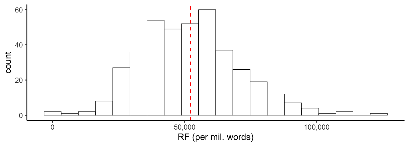
  theme(axis.text = element_text(size=5))

Histogram of the tokens the and of.

If we don’t want overlapping histograms, we can use facet_wrap() to split the plots.

ggplot(word_df,aes(x = RF, color = token, fill = token)) + 
  geom_histogram(binwidth = bin_width(word_df$RF), alpha=.5, position = "identity") +
  theme_classic() +
  theme(axis.text = element_text(size=5)) +
  theme(legend.position = "none") +
  xlab("RF (per mil. words)") +
  facet_wrap(~ token)

Histogram of the tokens the and of.

Pause for Lab Set Question

Complete Task 1 in Lab Set 2.

4.7 Dispersion

We can also calculate dispersion, and there are a variety of measures at our disposal. Our toolkit has several functions for producing these calculations.

For example, we can find the dispersion of any specific token:

the <- dispersions_token(sc_dfm, "the") %>% unlist()

Dispersion measures for the token .

Absolute frequency	50920.000
Per_10.5	5240.015
Relative entropy of all sizes of the corpus parts	1.000
Range	399.000
Maxmin	292.000
Standard deviation	45.926
Variation coefficient	0.361
Chi-square	6295.422
Juilland et al.’s D (based on equally-sized corpus parts)	0.982
Juilland et al.’s D (not requiring equally-sized corpus parts)	0.982
Carroll’s D2	0.989
Rosengren’s S (based on equally-sized corpus parts)	0.963
Rosengren’s S (not requiring equally-sized corpus parts)	0.966
Lyne’s D3 (not requiring equally-sized corpus parts)	0.968
Distributional consistency DC	0.963
Inverse document frequency IDF	0.004
Engvall’s measure	50792.700
Juilland et al.’s U (based on equally-sized corpus parts)	50000.333
Juilland et al.’s U (not requiring equally-sized corpus parts)	50010.750
Carroll’s Um (based on equally sized corpus parts)	50342.268
Rosengren’s Adjusted Frequency (based on equally sized corpus parts)	49032.932
Rosengren’s Adjusted Frequency (not requiring equally sized corpus parts)	49185.689
Kromer’s Ur	2135.564
Deviation of proportions DP	0.139
Deviation of proportions DP (normalized)	0.139

And let’s try another token to compare:

data <- dispersions_token(sc_dfm, "data") %>% unlist()

Deviation of Proportions for the tokens and .

	the	data
Deviation of proportions DP	0.139	0.846

Pause for Lab Set Question

Complete Task 2 in Lab Set 2.

4.7.1 Dispersions for all tokens

We can also calculate selected dispersion measures for all tokens using dispersions_all():

d <- dispersions_all(sc_dfm)

Dispersion measures for all tokens.

Token	AF	Per_10.5	Carrolls_D2	Rosengrens_S	Lynes_D3	DC	Juillands_D	DP	DP_norm
the	50920	5240.015	0.989	0.966	0.968	0.963	0.982	0.139	0.139
and	25232	2596.545	0.990	0.970	0.973	0.967	0.983	0.123	0.124
to	24753	2547.252	0.993	0.980	0.983	0.976	0.987	0.090	0.090
of	22060	2270.124	0.978	0.933	0.935	0.932	0.974	0.199	0.199
a	21614	2224.228	0.992	0.977	0.978	0.973	0.986	0.109	0.109
in	15969	1643.319	0.988	0.962	0.963	0.960	0.981	0.146	0.146

4.8 Generating a frequency table

Alternatively, frequency_table() returns only Deviation of Proportions and Average Reduced Frequency.

Note that ARF requires a tokens object and takes a couple of minutes to calculate.

ft <- frequency_table(sc_tokens)

Frequency and dispersion measures for all tokens.

	Token	AF	Per_10.5	ARF	DP
1	the	50920	5240.015	31901.106	0.139
2	and	25232	2596.545	15914.149	0.123
3	to	24753	2547.252	15468.494	0.090
5	of	22060	2270.124	13089.728	0.199
4	a	21614	2224.228	13239.704	0.109
6	in	15969	1643.319	9772.267	0.146

Pause for Lab Set Question

Complete Task 3 in Lab Set 2.

4.9 Zipf’s Law

Let’s plot rank against frequency for the 100 most frequent tokens in the sample corpus.

ggplot(freq_df %>% filter(rank < 101), aes(x = rank, y = frequency)) +
  geom_point(shape = 1, alpha = .5) +
  theme_classic() +
  ylab("Absolute frequency") +
  xlab("Rank")

Token rank vs. frequency.

The relationship you’re seeing between the rank of a token and it’s frequency holds true for almost any corpus and is referred to as Zipf’s Law (see Brezina pg. 44).

Pause for Lab Set Question

Complete Task 4 in Lab Set 2.