Examples Gallery

This gallery showcases complete workflows for common sentiment analysis tasks. Each example is self-contained and ready to adapt for your own projects.

Setup

from moodswing import (
    DictionarySentimentAnalyzer,
    Sentencizer,
    DCTTransform,
    prepare_trajectory,
    plot_trajectory,
    trajectory_to_dataframe,
)
from moodswing.data import load_sample_text
import matplotlib.pyplot as plt
import numpy as np
import pandas as pd

Example 1: Comparing multiple novels

Analyze and compare the emotional arcs of several novels side-by-side:

# Setup
sentencizer = Sentencizer()
analyzer = DictionarySentimentAnalyzer()

# Select novels to compare
novels = [
    "portrait_artist",
    "madame_bovary", 
    "ragged_dick"
]

# Create subplots
fig, axes = plt.subplots(1, 3, figsize=(15, 4), dpi=150, sharey=True)

for ax, novel_id in zip(axes, novels):
    try:
        # Load and process
        doc_id, text = load_sample_text(novel_id)
        sentences = sentencizer.split(text)
        scores = analyzer.sentence_scores(sentences, method="syuzhet")
        
        # Create trajectory
        trajectory = prepare_trajectory(
            scores,
            rolling_window=int(len(scores) * 0.05),
            dct_transform=DCTTransform(low_pass_size=5, output_length=200, scale_range=True)
        )
        
        # Plot only DCT
        plot_trajectory(trajectory, components=['dct'], title=doc_id, ax=ax)
        ax.set_xlabel('Narrative Position')
        if ax == axes[0]:
            ax.set_ylabel('Sentiment')
    except Exception as e:
        print(f"Could not process {novel_id}: {e}")

plt.tight_layout()
plt.show()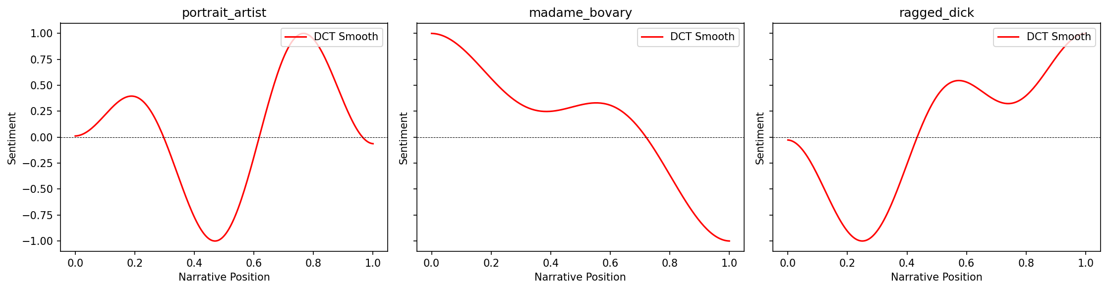

Example 2: Chapter-by-chapter analysis

Analyze a novel broken into chapters to see emotional patterns at the chapter level:

# Load a novel
doc_id, text = load_sample_text("portrait_artist")

# Split into chapters (using Chapter markers as delimiters)
import re
chapters = re.split(r'\s*Chapter\s+[IVXLC]+\s*', text)
chapters = [ch.strip() for ch in chapters if ch.strip()]

print(f"Found {len(chapters)} chapters in {doc_id}")

# Score each chapter
chapter_scores = []
for i, chapter in enumerate(chapters, 1):
    sents = sentencizer.split(chapter)
    scores = analyzer.sentence_scores(sents, method="syuzhet")
    avg_score = np.mean(scores) if scores else 0
    chapter_scores.append({
        'chapter': i,
        'mean_sentiment': avg_score,
        'sentences': len(sents),
        'std_sentiment': np.std(scores) if scores else 0
    })

# Create DataFrame
chapters_df = pd.DataFrame(chapter_scores)
print(chapters_df.head())

Found 5 chapters in portrait_artist
   chapter  mean_sentiment  sentences  std_sentiment
0        1       -0.033272       1366       0.812152
1        2        0.021910        801       1.024633
2        3       -0.419166        887       1.490579
3        4        0.087970        399       1.343594
4        5        0.093825       1919       0.887800

fig, (ax1, ax2) = plt.subplots(1, 2, figsize=(14, 4), dpi=150)

# Plot 1: Mean sentiment by chapter
ax1.bar(chapters_df['chapter'], chapters_df['mean_sentiment'], 
        color='steelblue', alpha=0.7, edgecolor='black')
ax1.axhline(0, color='black', linewidth=0.5, linestyle='--')
ax1.set_xlabel('Chapter Number', fontsize=11)
ax1.set_ylabel('Mean Sentiment', fontsize=11)
ax1.set_title('Average Sentiment by Chapter', fontsize=12, fontweight='bold')
ax1.grid(True, alpha=0.2, axis='y')

# Plot 2: Sentiment variability
ax2.bar(chapters_df['chapter'], chapters_df['std_sentiment'], 
        color='coral', alpha=0.7, edgecolor='black')
ax2.set_xlabel('Chapter Number', fontsize=11)
ax2.set_ylabel('Standard Deviation', fontsize=11)
ax2.set_title('Emotional Variability by Chapter', fontsize=12, fontweight='bold')
ax2.grid(True, alpha=0.2, axis='y')

plt.tight_layout()
plt.show()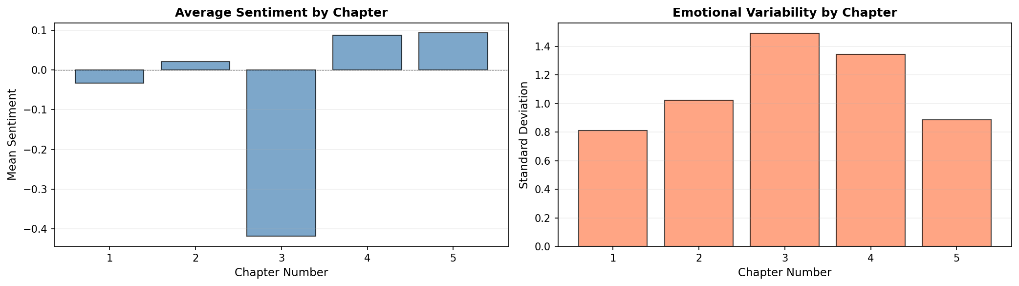

Example 3: Multi-dimensional emotion tracking

Track and visualize multiple NRC emotions simultaneously:

# Load and analyze
doc_id, text = load_sample_text("ragged_dick")
sentences = sentencizer.split(text)

# Get NRC emotions
emotions = analyzer.nrc_emotions(sentences)
emotions_df = pd.DataFrame(emotions)

# Sample every Nth sentence for cleaner visualization
sample_rate = max(1, len(emotions_df) // 100)  # ~100 points
emotions_sampled = emotions_df.iloc[::sample_rate]

# Select key emotions for heatmap
emotion_cols = ['joy', 'fear', 'anger', 'sadness', 'trust', 'anticipation', 'surprise', 'disgust']

# Create heatmap
fig, ax = plt.subplots(figsize=(12, 6), dpi=150)
im = ax.imshow(emotions_sampled[emotion_cols].T, aspect='auto', cmap='YlOrRd', interpolation='nearest')

# Customize
ax.set_yticks(range(len(emotion_cols)))
ax.set_yticklabels([e.title() for e in emotion_cols], fontsize=11)
ax.set_xlabel('Narrative Position (sampled)', fontsize=11)
ax.set_title(f'{doc_id}: Emotional Heatmap', fontsize=13, fontweight='bold')

# Add colorbar
cbar = plt.colorbar(im, ax=ax)
cbar.set_label('Emotion Intensity', rotation=270, labelpad=20, fontsize=11)

plt.tight_layout()
plt.show()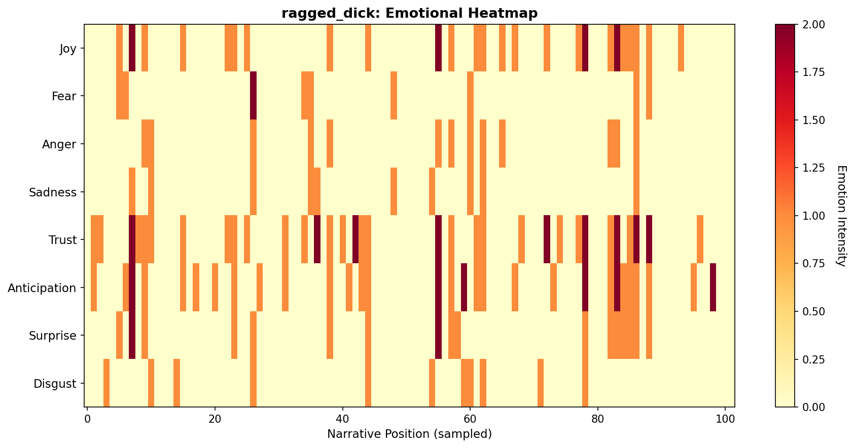

Example 4: Comparing sentiment methods

Compare how different lexicons score the same text:

doc_id, text = load_sample_text("madame_bovary")
sentences = sentencizer.split(text)

# Score with all four lexicons
methods = ['syuzhet', 'afinn', 'bing', 'nrc']
trajectories = {}

for method in methods:
    scores = analyzer.sentence_scores(sentences, method=method)
    traj = prepare_trajectory(
        scores,
        dct_transform=DCTTransform(low_pass_size=5, output_length=200, scale_range=True)
    )
    trajectories[method] = traj

# Plot comparison
fig, axes = plt.subplots(2, 2, figsize=(14, 8), dpi=150)
axes = axes.flatten()

colors = ['crimson', 'steelblue', 'green', 'orange']

for ax, method, color in zip(axes, methods, colors):
    traj = trajectories[method]
    x = np.linspace(0, 1, len(traj.dct))
    ax.plot(x, traj.dct, color=color, linewidth=2.5, label=method.upper())
    ax.axhline(0, color='black', linewidth=0.5, linestyle='--', alpha=0.3)
    ax.set_title(f'{method.upper()} Lexicon', fontsize=12, fontweight='bold')
    ax.set_xlabel('Narrative Position', fontsize=10)
    ax.set_ylabel('Sentiment', fontsize=10)
    ax.grid(True, alpha=0.2)
    ax.set_ylim(-1.1, 1.1)

fig.suptitle(f'{doc_id}: Lexicon Comparison', fontsize=14, fontweight='bold')
plt.tight_layout()
plt.show()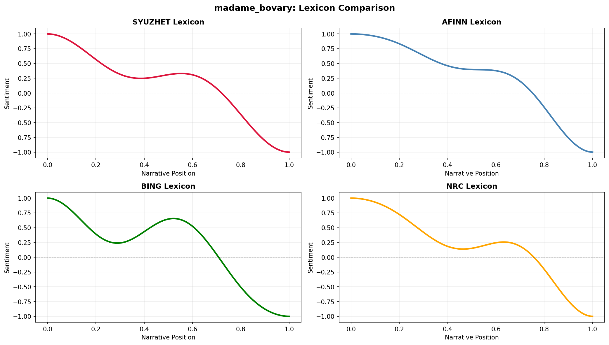

Comparing four lexicons on the same text

Example 5: Custom color schemes for themes

Create thematic color palettes for different genres or moods:

# Define color themes
themes = {
    'gothic': {'raw': '#2D2D2D', 'rolling': '#8B4513', 'dct': '#8B0000'},
    'romantic': {'raw': '#FFE4E1', 'rolling': '#FF69B4', 'dct': '#DC143C'},
    'modern': {'raw': '#E0E0E0', 'rolling': '#4A90E2', 'dct': '#50C878'},
}

# Load text
doc_id, text = load_sample_text("silas_lapham")
sentences = sentencizer.split(text)
scores = analyzer.sentence_scores(sentences, method="syuzhet")
trajectory = prepare_trajectory(
    scores,
    rolling_window=int(len(scores) * 0.05),
    dct_transform=DCTTransform(low_pass_size=5, output_length=200, scale_range=True)
)

# Plot with each theme
fig, axes = plt.subplots(1, 3, figsize=(15, 4), dpi=150)

for ax, (theme_name, colors) in zip(axes, themes.items()):
    plot_trajectory(trajectory, colors=colors, title=f'{theme_name.title()} Theme', ax=ax)
    ax.set_facecolor('#FAFAFA')

plt.tight_layout()
plt.show()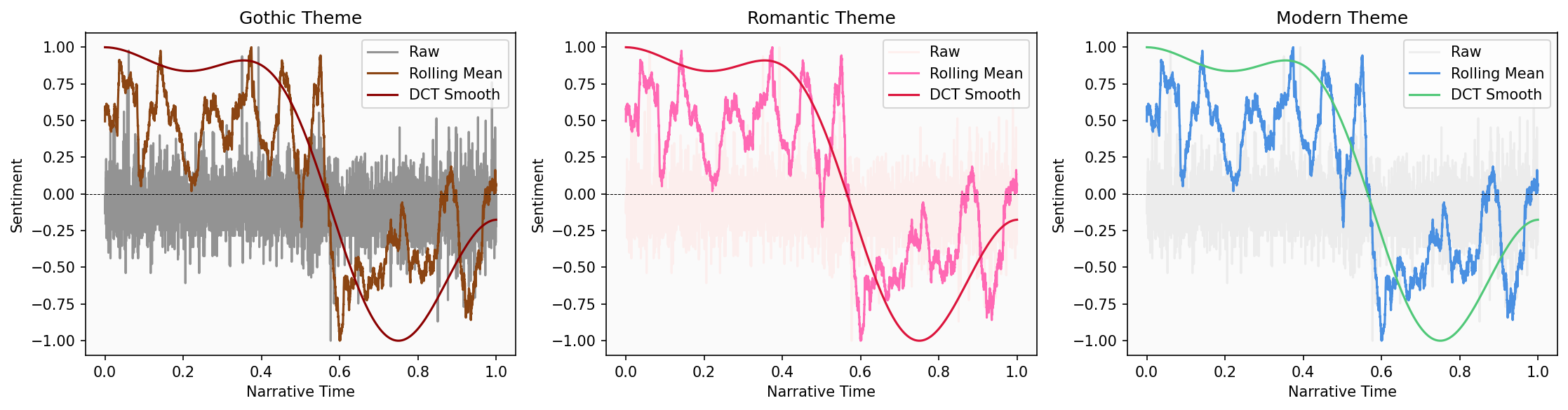

Example 6: Export data for external tools

Prepare sentiment data for analysis in R, Excel, or other tools:

# Full analysis pipeline with data export
doc_id, text = load_sample_text("madame_bovary")
sentences = sentencizer.split(text)

# Get multiple types of scores
syuzhet_scores = analyzer.sentence_scores(sentences, method="syuzhet")
emotions = analyzer.nrc_emotions(sentences)

# Create comprehensive DataFrame
analysis_df = pd.DataFrame({
    'sentence_num': range(1, len(sentences) + 1),
    'sentence_text': sentences,
    'syuzhet_score': syuzhet_scores,
})

# Add NRC emotions
emotions_df = pd.DataFrame(emotions)
analysis_df = pd.concat([analysis_df, emotions_df], axis=1)

# Add trajectory data (aligned to sentence positions)
trajectory = prepare_trajectory(
    syuzhet_scores,
    rolling_window=int(len(syuzhet_scores) * 0.05),
    dct_transform=DCTTransform(low_pass_size=5, output_length=len(sentences), scale_range=True)
)

analysis_df['raw_normalized'] = trajectory.raw
analysis_df['rolling_smooth'] = trajectory.rolling[:len(sentences)]
analysis_df['dct_smooth'] = trajectory.dct[:len(sentences)]

# Display sample
print(analysis_df.head())

   sentence_num                                      sentence_text  \
0             1  Part I Chapter One We were in class when the h...   
1             2  Those who had been asleep woke up, and every o...   
2             3     The head-master made a sign to us to sit down.   
3             4  Then, turning to the class-master, he said to ...   
4             5  If his work and conduct are satisfactory, he w...   

   syuzhet_score  anger  anticipation  disgust  fear  joy  negative  positive  \
0           1.20    0.0           0.0      0.0   0.0  0.0       1.0       1.0   
1           0.25    0.0           0.0      0.0   0.0  0.0       0.0       0.0   
2           0.00    0.0           0.0      0.0   0.0  0.0       0.0       0.0   
3           1.50    0.0           0.0      0.0   0.0  0.0       0.0       1.0   
4           1.05    0.0           0.0      0.0   0.0  0.0       0.0       0.0   

   sadness  surprise  trust  raw_normalized  rolling_smooth  dct_smooth  
0      0.0       0.0    4.0       -0.068702        0.481874    1.000000  
1      0.0       1.0    0.0       -0.213740        0.449076    0.999999  
2      0.0       0.0    0.0       -0.251908        0.462119    0.999998  
3      0.0       0.0    1.0       -0.022901        0.463712    0.999996  
4      0.0       0.0    0.0       -0.091603        0.459667    0.999994

# Export
analysis_df.to_csv(f'{doc_id}_full_analysis.csv', index=False)
analysis_df.to_excel(f'{doc_id}_full_analysis.xlsx', index=False)

print(f"\\nExported {len(analysis_df)} sentences with {len(analysis_df.columns)} features")
print("Files created: CSV and Excel formats")

Example 8: Progressive trajectory reveal

Visualize how a narrative arc unfolds over time using a grid of progressive snapshots:

# Create progressive reveal visualization
doc_id, text = load_sample_text("portrait_artist")
sentences = sentencizer.split(text)
scores = analyzer.sentence_scores(sentences, method="syuzhet")

# Create full trajectory
full_trajectory = prepare_trajectory(
    scores,
    dct_transform=DCTTransform(low_pass_size=5, output_length=200, scale_range=True)
)

positions = np.linspace(0, 1, len(full_trajectory.dct))

# Create grid of 10 frames (2 rows x 5 columns)
fig, axes = plt.subplots(2, 5, figsize=(16, 6), dpi=150)
axes = axes.flatten()

n_frames = 10
for frame_num, ax in enumerate(axes, 1):
    # Show first N% of trajectory
    cutoff = int(len(positions) * (frame_num / n_frames))
    
    # Plot progressive portion
    ax.plot(positions[:cutoff], full_trajectory.dct[:cutoff], 
            color='crimson', linewidth=2)
    ax.axhline(0, color='black', linewidth=0.5, linestyle='--', alpha=0.3)
    ax.set_xlim(0, 1)
    ax.set_ylim(-1.1, 1.1)
    
    # Minimize labels for grid view
    ax.set_title(f'{frame_num*10}%', fontsize=10, fontweight='bold')
    ax.tick_params(labelsize=7)
    ax.grid(True, alpha=0.2)
    
    # Only show axis labels on outer edges
    if frame_num > 5:
        ax.set_xlabel('Position', fontsize=8)
    if frame_num in [1, 6]:
        ax.set_ylabel('Sentiment', fontsize=8)

fig.suptitle(f'{doc_id}: Progressive Arc Development', fontsize=14, fontweight='bold')
plt.tight_layout()
plt.show()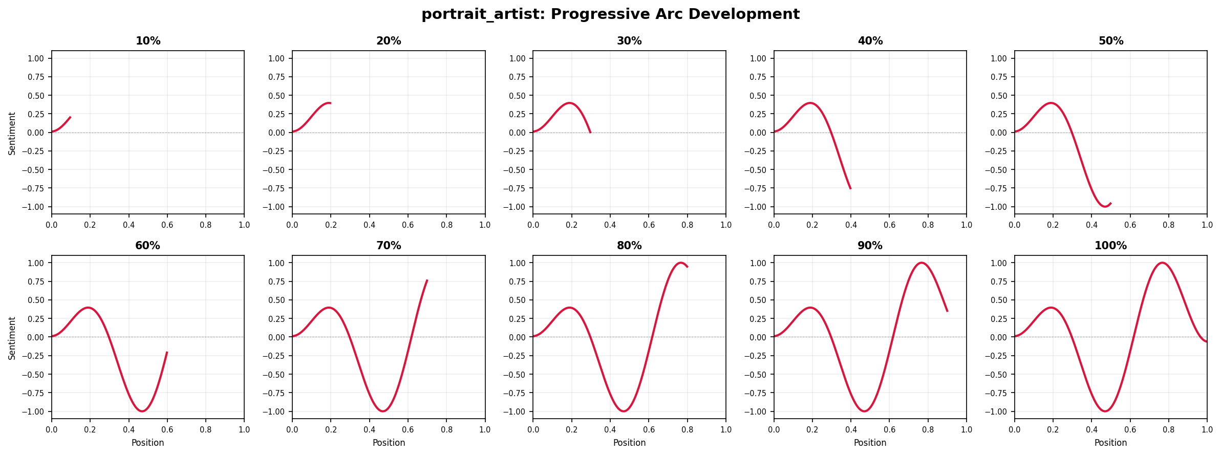

Progressive reveal showing narrative arc development from 10% to 100%

This “storyboard” view shows how the emotional trajectory emerges gradually—useful for presentations or for understanding when key narrative shifts occur.

Next steps

Adapt these examples for your own texts
Combine techniques for richer analysis
See Visualization Guide for more styling options
Read Technical Notes for implementation details