Cluster Analysis

Fall 2025
Two types of cluster analysis
- Hierarchical agglomerative clustering
- \(K\)-means clustering
Hierarchical clustering
Hierarchical clustering
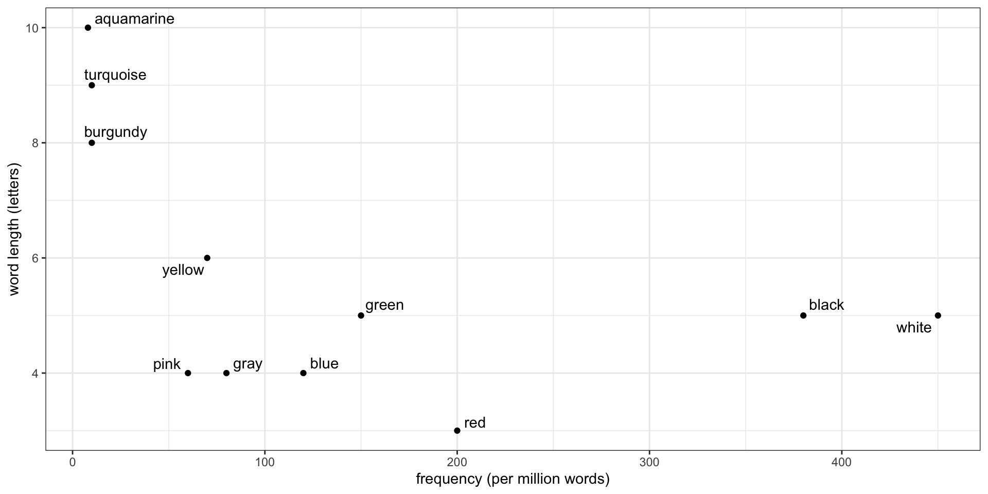
Standardize the data
\[ z = \frac{\text{value} - \text{mean}}{\text{standard deviation}} \]
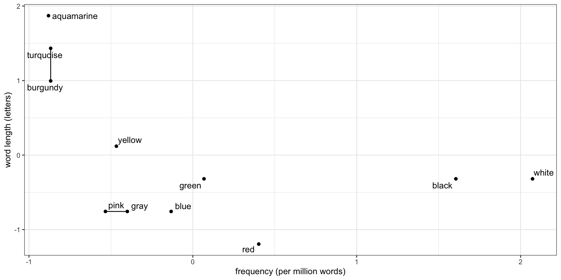
Standardized data
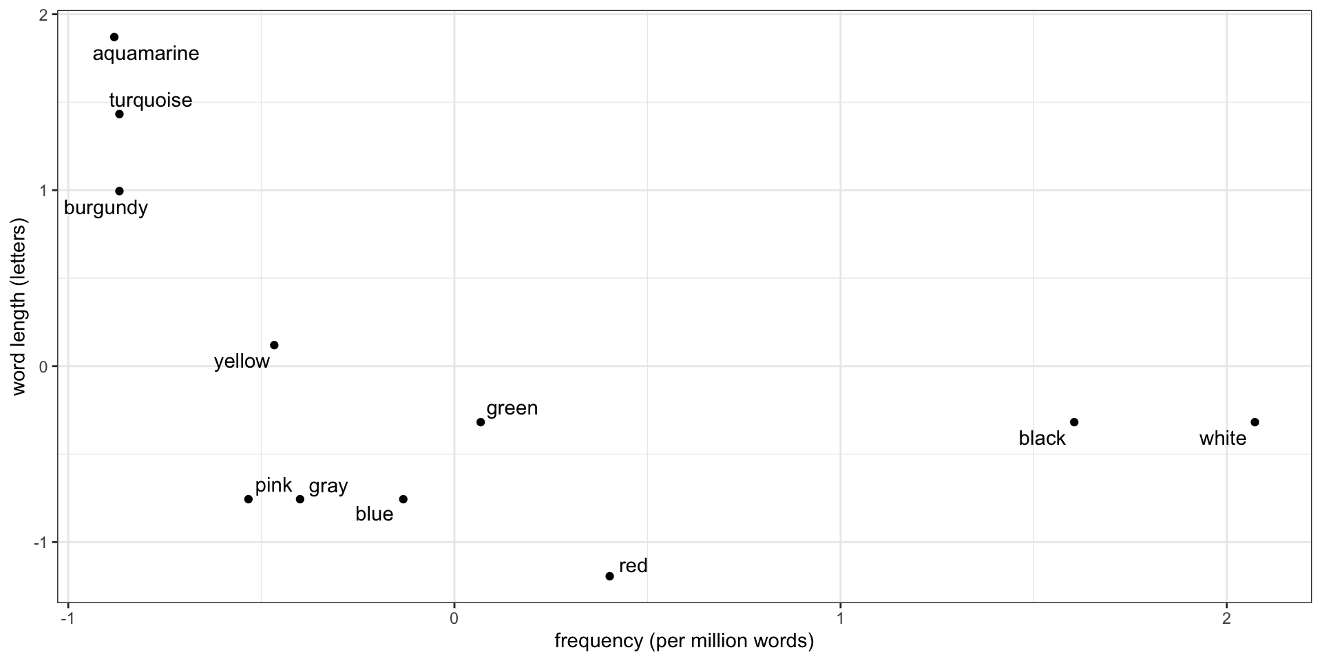
Clustering requires distances
- To cluster, group nearby points
- What does “nearby” mean? Options:
- Euclidean distance: \[\begin{align*} \operatorname{dist}(a, b) &= \sqrt{(a_x - b_x)^2 + (a_y - b_y)^2} \\ &= \|a - b\|_2 \end{align*}\]
- Manhattan distance: \[\begin{align*} \operatorname{dist}(a, b) &= |a_x - b_x| + |a_y - b_y| \\ &= \|a - b\|_1 \end{align*}\]
Find the closest pair of points
Euclidean \(\operatorname{dist}(\text{pink}, \text{gray}) = 0.13\)
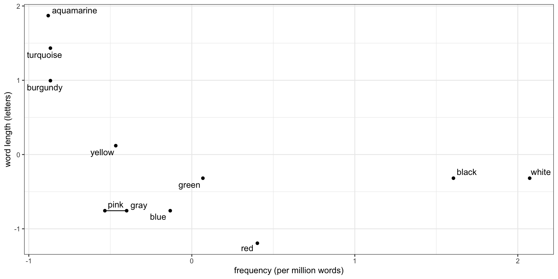
Then find the next closest
But how close is a point to a cluster?
How close is blue to the pink-gray cluster? How we measure this is called the linkage:
- Distance from blue to the nearest point in the cluster: single linkage
- Distance from blue to the farthest point in the cluster: complete linkage
- Average distance from blue to each point in the cluster: average linkage
- Change in squared distances within the clusters: Ward’s method
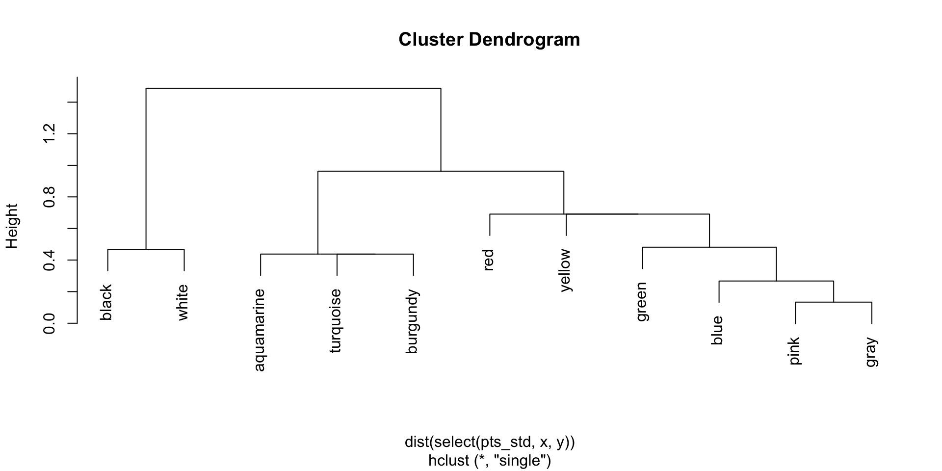
Single linkage dendrogram
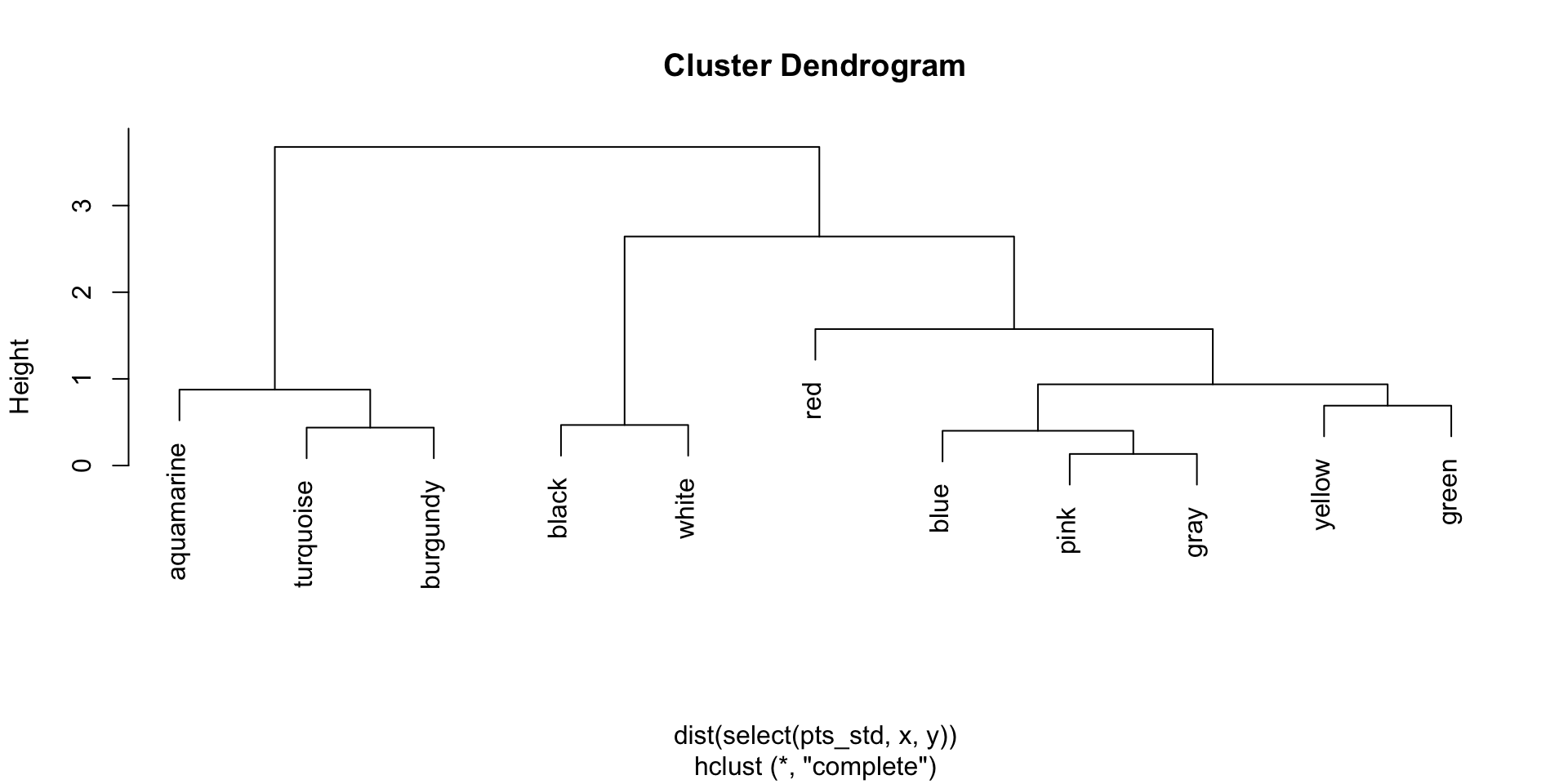
Complete linkage dendrogram
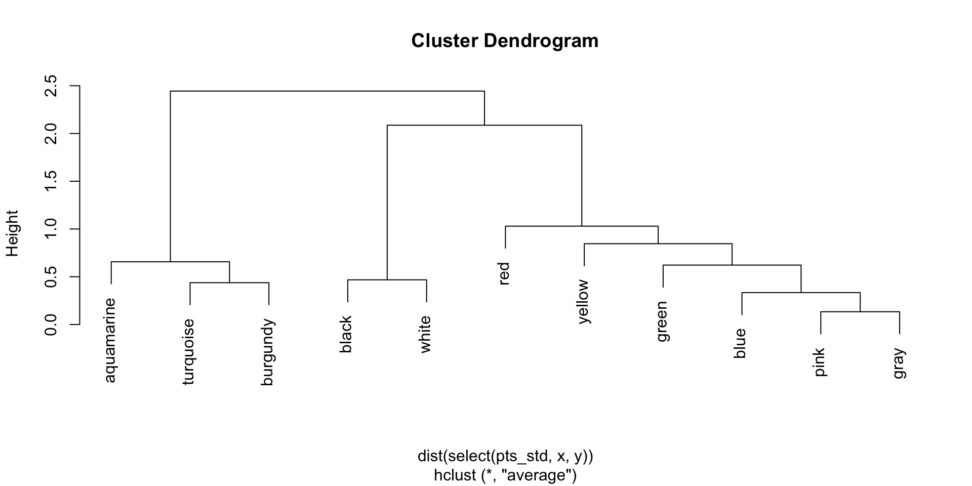
Average linkage dendrogram
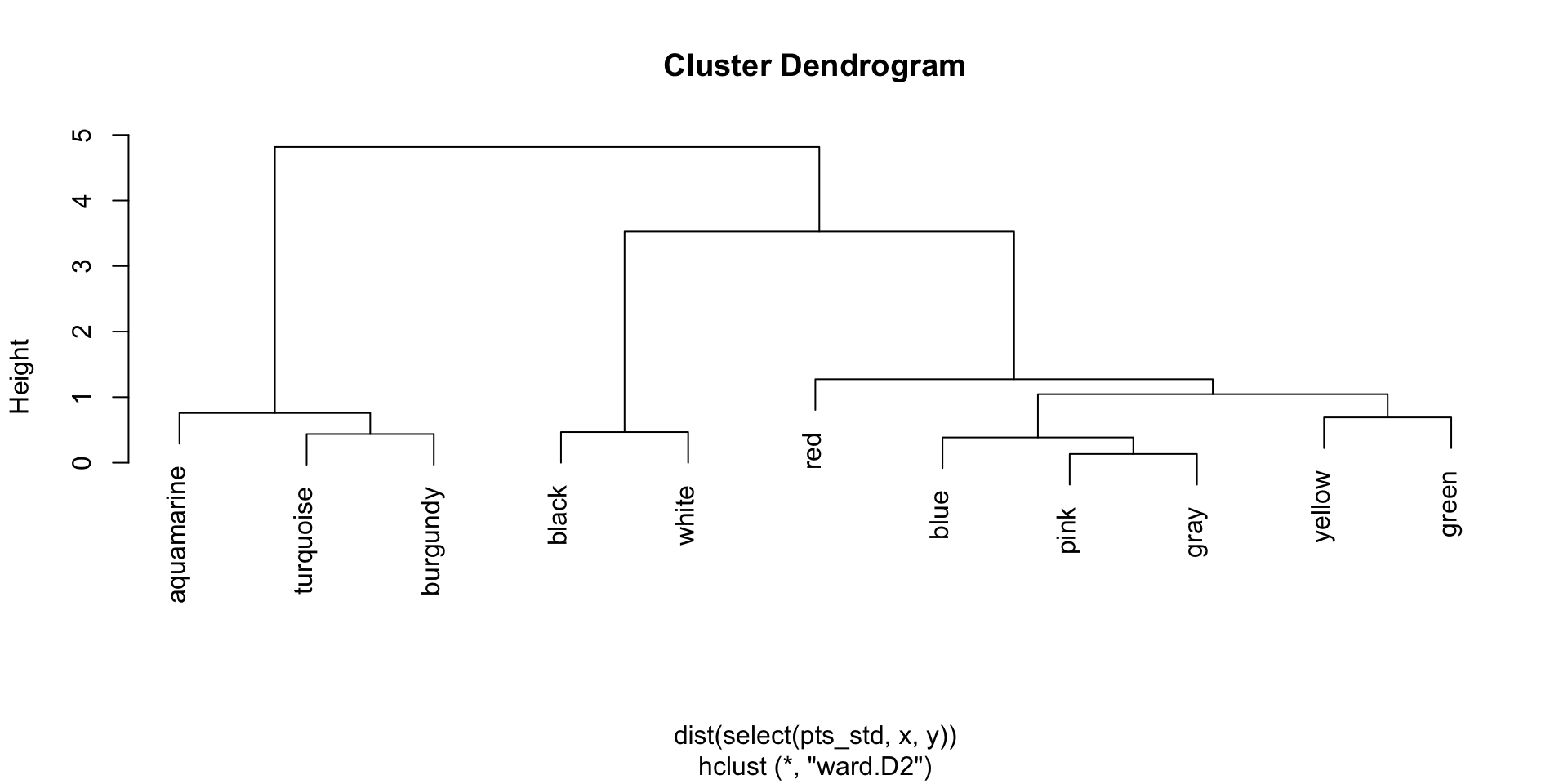
Ward’s linkage dendrogram
There is no single correct clustering
- Clustering is an unsupervised method: we group observations with similar attributes
- There is no response variable, so this is not a classification problem
- Hence there is no “right” answer
- The purpose of clustering is interpretation: finding similar observations so we can discuss them as a group
Measuring the amount of clustering
- Let \(l(i)\) be the distance between word \(i\) and the first cluster/word it was merged with
- If \(l(i)\) is small, it was similar to another word; if \(l(i)\) is large, it was only grouped later
- Let \(l_\text{max} = \max_i l(i)\)
Then the agglomerative coefficient is: \[ \text{AC} = \frac{1}{n} \sum_{i=1}^n \frac{l_\text{max} - l(i)}{l_\text{max}} = \frac{1}{n} \sum_{i=1}^n \left(1 - \frac{l(i)}{l_\text{max}} \right) \]
- \(\text{AC} \approx 0\): little cluster structure, words merged late
- \(\text{AC} \approx 1\): lots of cluster structure, many words merged early
Reporting a clustering analysis
- Cluster analysis is largely an exploratory visual method to show patterns in the data.
- The parameters for cluster identification (data transformation, distance measure, cluster combination method) need to be reported.
- The Methods section should describe the analytical procedure and the parameters used.
- In the Results and Discussion, each tree plot (dendrogram) needs to be carefully discussed.
How many meaningful factors be observed in the plot?
K-means clustering
K-means clustering
- \(K\)-means clustering works on a different principle: instead of hierarchically joining clusters, fix the number (\(K\)) in advance
- Then choose clusters such that points within the cluster are similar to each other compared to points outside the cluster
That is, we find:
- \(K\) cluster centers, \(\mu_1, \mu_2, \dots, \mu_K\)
- Cluster assignments placing every observation in cluster \(1, 2, \dots, K\)
The objective
To find the cluster centers, we want to minimize the within-cluster variation. Let \(C_k\) be the set of observations in cluster \(k\): \[ W(C_k) = \sum_{i \in C_k} \|x_i - \mu_k\|_2^2 \]
The total within-cluster variation is \[ \sum_{k = 1}^K W(C_k) \]
We want to minimize this by choosing \(\mu_k\) and \(C_k\).
The optimization is hard
- Actually optimizing the within-cluster variation is hard: there is a huge number of possible cluster assignments
- (You can do the combinatorics)
- Because cluster assignment is discrete, you can’t just take the derivative and set to zero to find the minimum
- …and you can’t use gradient descent or any numerical optimizer
- The actual optimization is NP-hard
- But we can approximate it!
The usual K-means algorithm
- Choose \(K\)
- Select \(K\) distinct observations from the data and make these the initial cluster centers \(\mu_1, \dots, \mu_K\)
- Set the cluster assignments \(C_k\) to assign each observation to the nearest center (based on Euclidean distance)
- Update the cluster centers to be the mean of the observations assigned to that cluster
- Return to step 3
Eventually this will converge to a local optimum and you can stop
How do we choose K?
- Again, this is an unsupervised problem, so there is no “correct” \(K\)
- When data is 2D, you can eyeball the plot and judge the number of clusters
- When data is 60D, you will find that difficult
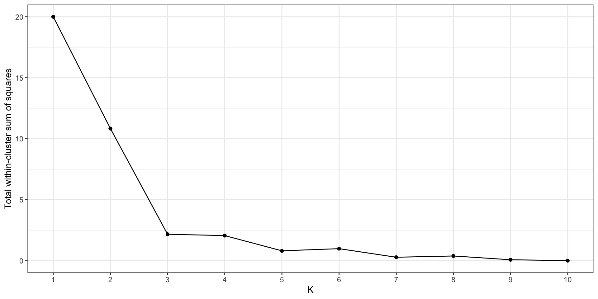
- You can try to minimize within-cluster variation, but…
- …the minimum is 0, when \(K = n\)
The elbow method
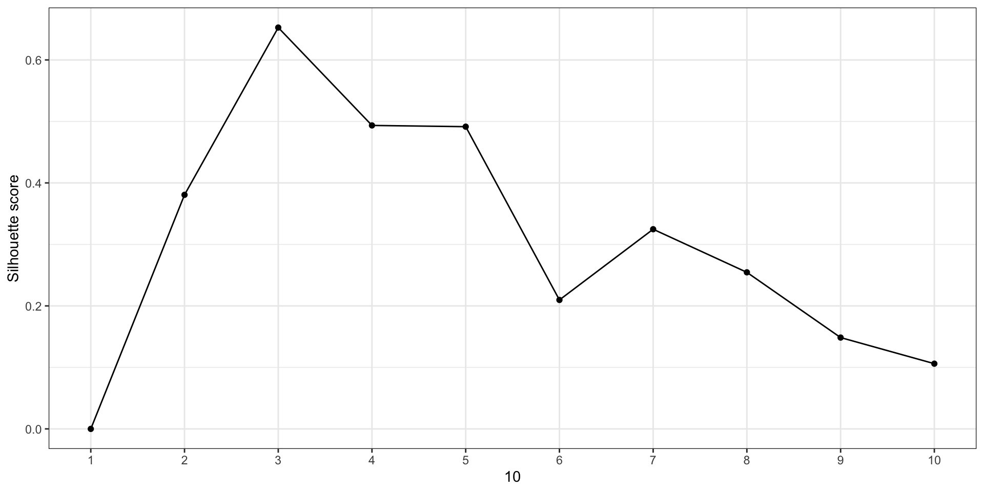
Silhouette method
- For each observation \(i\), let
- \(a(i) = {}\) mean distance between \(i\) and all other points in the same cluster
- \(b(i) = {}\) mean distance between \(i\) and all points in the nearest other cluster
Then \[ s(i) = \frac{b(i) - a(i)}{\max\{ a(i), b(i) \}} \] (or 0 if no other points in the same cluster)
Average of \(s(i)\) is the silhouette score
Silhouette method